
Research
Sampling & particle methods
In machine learning, models are trained by finding parameters that make a loss small. But several different explanations may fit the same data, and a single fitted model can hide that uncertainty. Sampling lets us explore these possibilities and average their predictions. This is central to Bayesian inference, uncertainty quantification, and generative modeling. The same idea appears in statistical physics, where samples describe the molecular configurations a system is likely to visit.
In my paper with Maarten de Hoop, we introduce a sampling method with a finite measure of error that decreases along particle motion (called Green–Bessel). This particle Lyapunov energy lets us prove last-iterate convergence: as the number of particles and observation time grow, the particle cloud approaches the target. Last-iterate convergence is well established for Langevin dynamics and is known for some special deterministic systems. Our contribution is to obtain it for a deterministic interacting-particle method with general smooth strictly positive targets on a compact state space, including multimodal targets, without time averaging, added noise, or log-concavity. The particles may start far from equilibrium, and the approximation is controlled uniformly over all time. Green–Bessel is also expected to explore the target’s modes much more quickly than classical Langevin dynamics or standard SVGD.
Background: Langevin, SVGD, LAWGD, and Green–Bessel
From gradient descent to sampling
Think of x as a possible set of model parameters and U(x) as a loss landscape. Gradient descent moves downhill. Sampling explores the whole landscape according to a target density π(x) = Z−1e−U(x), where Z makes the density integrate to one. Low-loss regions receive more weight, while their width and volume also matter. For Bayesian inference, U is the negative log-likelihood plus the negative log-prior; in a Gibbs model, it is physical energy scaled by temperature.
Stochastic gradient descent (SGD) already has randomness because it estimates gradients from minibatches. For small learning rates, sufficiently smooth losses, and independently sampled minibatches with unbiased gradient estimates, finite variance, and controlled higher moments, its finite-time statistics can be approximated by a diffusion (Li, Tai & E). Langevin dynamics gives a particularly clean version of this idea: gradient descent with calibrated Brownian noise.
Here Xi is one evolving candidate, t is time, ∇ is the gradient, and the Bi are independent Brownian motions. The noise helps candidates explore beyond the nearest minimum. Sampling can use one trajectory observed over time, or many trajectories run together. In the particle methods below, a whole cloud represents the distribution and its members interact to improve coverage.
How close is this to ordinary SGD?
Ordinary SGD’s minibatch noise generally depends on the current parameters and has different strengths in different directions, so it does not automatically sample π. Diffusion models of SGD are useful approximations under assumptions on stepsizes and noise (Mandt, Hoffman & Blei). Stochastic gradient Langevin dynamics explicitly adds noise to minibatch updates to target a posterior, with suitable stepsize control (Welling & Teh).
The density ρt of Langevin candidates relaxes toward π. Relative entropy Ht = KL(ρt|π) measures distributional error and decreases along this population flow.
Population flow, Fisher information I, and entropy
Ht = KL(ρt|π) is the relative entropy, ∫ρt log(ρt/π) dx. The relative Fisher information I = ∫|∇log(ρt/π)|2ρt dx measures mismatch in density gradients. The exponential bound holds when the target has log-Sobolev constant CLS. See the Langevin gradient-flow viewpoint.
Why separated modes are slow
Write the relative density error as u = ρ/π − 1. The Fokker–Planck equation becomes a linear equation for u, introducing the nonnegative Langevin operator Aπ:
The eigenfunctions ϕk are natural error patterns, ak(0) their initial amplitudes, and λk their decay rates. Below, the first eigenfunction is nearly constant within each well, with opposite signs. This missing-well imbalance relaxes slowly because λ1 is small: Langevin particles rarely cross the low-density gap, so exchanging probability between wells takes a long time.
A two-well target
The slow missing-well error
SVGD: move a cloud together
Stein variational gradient descent (SVGD) moves particles deterministically, using kernel interactions to spread them out. The kernel k(x,y) couples states x and y. With N particles,
These terms combine attraction toward probability mass and particle repulsion; ∇2 differentiates the second kernel argument. This is gradient descent over distributions (Liu & Wang; Liu).
Population flow and kernel Stein discrepancy (KSD)
The velocity vρ replaces the particle average by an average over the current distribution ρ. KSDk, the kernel Stein discrepancy, is the size of this velocity in the kernel’s space of vector fields:
Here d is the state dimension and ℋkd is the vector-valued reproducing-kernel Hilbert space generated by k; its norm measures the size of a field using that kernel. The discrepancy vanishes at the target. Equivalently, it is the largest average Stein residual ∇·g + g·∇log π among vector fields g of kernel norm at most one.
LAWGD (Laplacian Adjusted Wasserstein Gradient Descent): give slow errors a boost
LAWGD weights each error component by 1/λk, giving slow, missing-well errors a boost. This “preconditioned Langevin” flow balances relaxation rates near the target, much as preconditioning accelerates an ill-conditioned optimization problem.
Its population entropy decays at a rate independent of the Poincaré constant, the target’s slow-relaxation timescale (Chewi and collaborators):
Here χ2(ρ|π) = ∫(ρ/π − 1)2dπ is the squared density-ratio error.
LAWGD flow
The Green kernel G0 implements the inverse of Aπ using the centered target eigenfunctions. Its particle and population velocities are
The density follows the same continuity equation as above. The entropy bound assumes a positive spectral gap and regular population solutions.
Green–Bessel: an energy for actual particles
We want a finite, decreasing energy for the actual particle cloud. LAWGD’s Green energy diverges on point masses in state dimension d ≥ 2. We retain its Green factor, 1/λk, and add Bessel smoothing for high-frequency errors:
Here μ is the current distribution; brackets compare averages of ϕk under μ and π, and r sets the smoothing strength. Sufficient smoothing makes the energy finite on particles, while it still vanishes exactly at the target. Its gradient flow gives
The empirical distribution μtN puts mass 1/N at each particle. This is our particle Lyapunov functional: once its energy is low, it stays low. It provides the uniform long-time control needed for the last-iterate particle convergence result described above.
Population dissipation and scope
A positive matrix-valued kernel realizes this gradient flow as SVGD. The complete theorem assumes a smooth strictly positive target on a compact connected manifold without boundary, sufficiently large integer r, and independent initialization from a fixed smooth density. It therefore covers periodic targets with multiple wells. The Euclidean extension needs additional regularity and transport estimates.
Earlier last-iterate results include Langevin diffusions, Langevin-regularized SVGD, and special deterministic Gaussian systems. Langevin guarantees concern convergence of the sampling law; they do not require a discrepancy that decreases along every realized particle cloud. The advance here combines deterministic dynamics, general smooth positive compact-state targets, initialization away from equilibrium, and control of arbitrarily late times. The original LAWGD analysis provides a population guarantee; a comparable general last-iterate particle theorem is not supplied there.
A finite, decreasing particle discrepancy is not unprecedented across all sampling methods: MMD gradient flows provide an earlier example. Their formulation uses target kernel averages, which can be approximated from target samples, and a decreasing discrepancy alone does not guarantee global convergence. Our contribution is the particular target-adapted particle energy and the joint long-time, many-particle convergence theorem it enables.
The numerical energy retains 256 spectral modes of Aπ for this four-well target.
Below, the same Green–Bessel energy is tracked for all four samplers—Green–Bessel SVGD, RBF SVGD, LAWGD, and Langevin dynamics—using the same target and initial particles. The plotted Em is a finite spectral approximation of this energy.
Green–Bessel and LAWGD both discover modes rapidly, but Green–Bessel deliberately weakens within-mode exploration through smoothing. This smoothing makes its energy finite on particle distributions.
Playback timing
Transient shows t = 0–0.3 in 10 screen seconds. Late Stage shows t = 0.3–600 in another 10 screen seconds. Each view has a constant speed and uses the same physical clock for all four samplers. Langevin updates 10 times per screen second in both views, using actual saved positions without fading. Its integration step and noise strength are unchanged.
Green–Bessel SVGD
RBF SVGD
LAWGD
Langevin dynamics
Full discrepancy history
Simulation setup
N = 64 particles. The target energy is U(x) = ∑j=1,2[(xj2−1)2/(2σ2) + xj2/2], where x = (x1, x2) and σ = 0.3 controls well sharpness. The numerical domain is [−1.9,1.9]2. Green–Bessel: smoothing strength r = 2.05 and length ℓ = 0.1. RBF: adaptive median-bandwidth multiplier 5.33484, selected using an independent sampling discrepancy.
The numerical energy uses weights 1/[λ(1+ℓ2λ)r], where ℓ = 0.10 is an adjustable smoothing length. The formula above uses the paper’s convention ℓ = 1. This reflecting-box example with r = 2.05 illustrates the method; the full theorem assumes a compact manifold without boundary and a larger smoothing exponent. Spectral resolution must also increase for an exact target limit.
LAWGD uses the same target eigenfunctions with inverse-eigenvalue weights; RBF uses a Gaussian kernel. Langevin uses independent Brownian noise, with integration step at most 0.001. All four clouds start from exactly the same positions and use the same target and physical time. Playback has a constant physical-time rate throughout each view; it never accelerates near the end. Langevin shows actual saved particle positions at discrete time steps, with constant opacity and no cross-fading. The transient and late stage each take 10 screen seconds, at constant rates of 0.03 and 59.97 physical time units per screen second, respectively. The noise strength is unchanged. The discrepancy plot shows the energy history through t = 600.
We are also developing full-waveform inversion (FWI) algorithms for inferring subsurface parameters from wave observations (work in preparation).
Learning physical operators
How can a learned model predict the evolution of a physical system across different initial states and resolutions? I study neural operators for kinetic, fluid, and wave dynamics, with the goal of building reusable, structure-preserving models for physical simulation.
Stochastic jump transformer
A standard transformer moves each token to a new state. A physical collision, however, can have several possible outcomes even for the same incoming pair. In work with Maarten de Hoop, we introduce the stochastic jump transformer: attention updates the context, a learned interaction rate determines whether a pair interacts, and a learned jump map determines the outcome. Randomness is part of the interaction law, rather than an approximation to deterministic attention.
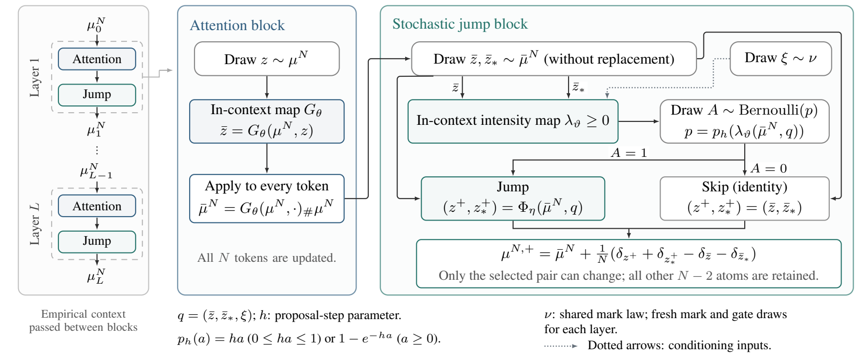
This gives a kinetic route to physics foundation models: learn local interaction laws and compose them across particles and time. The architecture can encode physical structure directly; for example, elastic pair maps preserve momentum and energy exactly. Our theory characterizes the continuous conditional laws represented by the architecture and connects small-step compositions to nonlinear drift–jump dynamics. Spatially mollified Maxwell–Boltzmann dynamics provide a concrete physical example.
T. Teolis and M. V. de Hoop. In-context Maps as a Collision Operator: Stochastic Jump Transformer. Preprint.
Markov Kernel Networks
Neural operators should respond stably when the same physical input is sampled on a different grid or point cloud. With David Mis, I. Dokmanić, Matti Lassas, and Maarten de Hoop, we develop Markov Kernel Networks as a common framework for transformers, Fourier neural operators, Flowers, and their hybrids. The networks alternate spatial information mixing through Markov kernels with pointwise channel mixing.
Our representation theorem characterizes uniformly discretization-stable operators as stable Markov Kernel Networks. A variational description of the read kernels then gives a way to recover familiar architectures and design new combinations. We are developing and training hybrid models at scale on acoustic wave datasets, with applications to wave propagation, Helmholtz equations, and inverse problems.
S. D. Mis, T. Teolis, I. Dokmanić, M. Lassas, and M. V. de Hoop. All Roads Lead to Markov Kernel Networks: A Representation Theorem for Discretization-Stable Learning. Preprint. Related work: Hybrid operator learning of wave scattering maps in high-contrast media.
Collective dynamics
Transformer inference dynamics
What happens to a prompt’s token representations as they pass through a transformer? In work with Sixu Li, Thomas Jacob Maranzatto, Jan Peszek, Semih Akkoc, Konstantin Riedl, Sennur Ulukus, and Nicolás García Trillos, we study these inference dynamics through interacting particle systems and collective dynamics. Attention mixes information between tokens; repeated mixing can produce clusters, collapse, or persistent motion. Understanding these patterns helps us ask what information a deep network preserves.
Here each particle xk is a token embedding on the unit circle, n is the number of tokens, and time t represents depth. We hold the learned maps fixed across layers and take a continuous-depth limit. The matrix A combines the query and key maps, while V is the value map. Softmax attention uses normalized exponential similarity weights αkj:
The brackets are Euclidean dot products. The tangent projection Px⊥y = y − ⟨x,y⟩x keeps embeddings on the circle and models layer normalization through a fixed-norm constraint. For linear attention, we replace the exponential by the dot product and use the fixed normalization n:
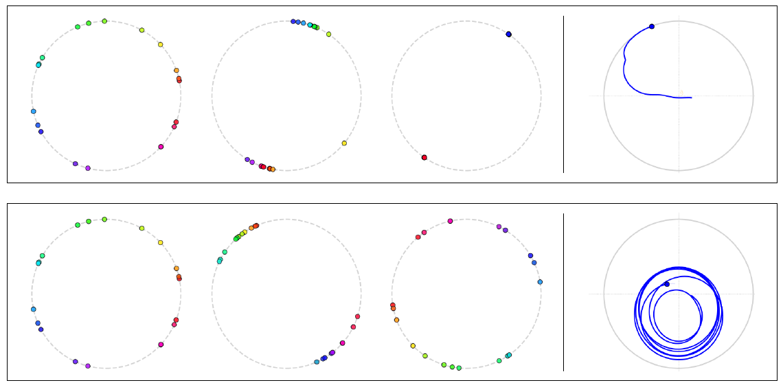
The top row shows the clustering regime; the bottom shows the oscillatory regime. A simple matrix family that captures this contrast is
Here I2 is the 2 × 2 identity matrix, a > 0 sets directional stretching, and b > 0 sets rotation. In this family, stronger stretching (a > b) gives the clustering regime, while stronger rotation (b > a) supports persistent oscillations.
The right-hand plots track R2, an order parameter for consensus along an axis. Here θj is token j’s angle and i is the imaginary unit. Its magnitude approaches 1 when tokens gather along a common axis, including two opposite clusters.
From my PhD: collective dynamics and fluid limits
How does coordinated motion emerge from local interactions? Collective dynamics involves flocking, swarming, synchronization, and self-organization. During my PhD, I studied how individual interactions become collective motion and how large particle systems turn into fluid equations, involving kinetic theory, multiscale modeling, and the emergence of macroscopic behavior.
Particles suspended in a fluid
The Fokker–Planck–Navier–Stokes (FPNS) system couples moving particles to a viscous, incompressible fluid. Particles align through Cucker–Smale interactions, feel drag and thermal noise, and push back on the fluid. In work with my advisor, Roman Shvydkoy, we use hypocoercivity to prove exponential synchronization for the locally smoothed drag model: the fluid approaches a constant velocity and the particle distribution approaches a Maxwellian centered at the same velocity. This holds without a small-initial-data assumption or an additional assumption that the evolving solution stays uniformly controlled for all time; the needed bounds follow from the model and the initial-data conditions.
The coupled equations
f(t,x,v) is the particle density in position x and velocity v; u is fluid velocity and p pressure. The communication kernel is φ, and sf(x) = ∫φ(x−y)f(y,w) dy dw is the local interaction strength. Subscript ε denotes spatial smoothing. The positive constants α, β, γ, ν, and σ control alignment, drag, fluid response, viscosity, and temperature. The theorem assumes a smooth nonnegative kernel of the form φ = ψ * ψ on a periodic domain, together with finite-energy and velocity-moment conditions.
Particles and fluid
Continuous particle paths across periodic cells; triangles point along their motion and blue arrows show the periodically repeated fluid. Thermal motion persists around the shared mean.
Simulation setup
The kinetic Fokker–Planck part is approximated by 96 stochastic particles: their positions follow their velocities, and their velocities evolve under alignment, fluid drag, and Brownian kicks representing velocity diffusion. These particles exchange momentum with a 24 × 24 incompressible Fourier fluid grid on the periodic unit square. Communication and two-way drag are spatially smoothed. A nonzero bulk drift and low positive temperature σ = 0.0004 make the shared direction visible. The integration step is 0.002, checked against 0.004 with coupled Brownian increments. The fluid field is projected to remain divergence-free; particle–fluid momentum exchange is balanced.
Hydrodynamic limits: from many velocities to a fluid
A hydrodynamic limit replaces a detailed distribution of particle positions and velocities by a few fields, such as density and fluid velocity. The idea comes from deriving fluid equations from molecular motion: local interactions act much faster than the large-scale flow, so they quickly establish a local equilibrium.
For an aligning population, rapid local relaxation pulls nearby velocities toward their local mean. If thermal noise also vanishes, the natural equilibrium has one velocity at each position: a monokinetic distribution. This is the cold, pressureless counterpart of the Maxwellian equilibrium used in gas dynamics. Writing ρ for density, u for velocity, and δu for a point mass at u, the limit f → ρδu leads to pressureless Euler alignment.
With Alina Chertock and Roman Shvydkoy, we ask a finer question: what shape survives inside the narrowing velocity distribution? The profile g(t,x,ξ) is that distribution viewed under a magnifying glass: ξ measures velocity relative to a moving local center, divided by its shrinking width. The density is rescaled to preserve mass. With vanishing noise and strong relaxation, its velocity shape becomes Gaussian; without noise, it obeys a transport equation and remembers its initial shape. These results use regularity and non-oscillation assumptions.
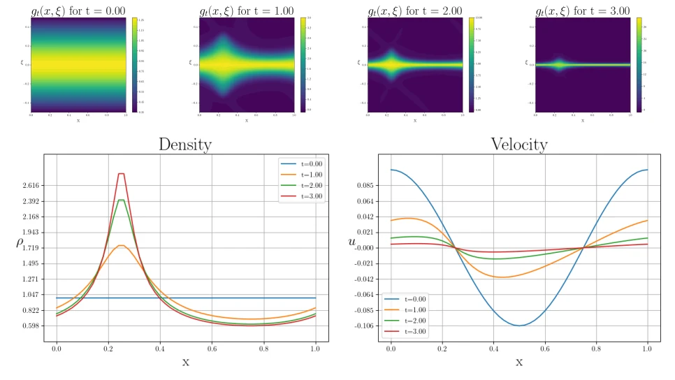
Asymmetric initial velocity
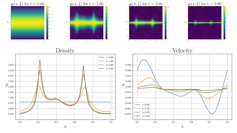
The s-model: adaptive communication strength
In the s-model, interaction strength is an evolving field s, allowing a flock to adapt its communication. With Roman Shvydkoy, we built the particle and kinetic descriptions and established their mean-field and hydrodynamic limits. The result connects individual agents to Euler-type fluid equations, in both the monokinetic and Maxwellian regimes.
Particles + strength field → Kinetic density + strength field → Euler alignment + strength field
How does communication strength shape collective motion in populations of different sizes and masses? These two simulations start from identical particles, with a small flock far from a much heavier one. In Cucker–Smale, the small flock spreads with little internal alignment. In the s-model, adaptive communication strength allows it to align locally while remaining far from the heavy flock.
Cucker–Smale
s-model: adaptive strength
Particle simulation setup
This recreates the qualitative experiment, not its exact initial data: 56 heavy and 8 light agents on the periodic unit square, each heavy agent having 100 times the mass of a light agent. As in the paper, φ(r) = (1+r²)−40 and alignment strength is 10. The adaptive model starts with s = 1. Its equivalent weight w = s/(φ * ρ) is transported by the locally averaged velocity, with initial w = 1/(φ * ρ). We evolve that field on a grid but display only particles. The strength field is not frozen or replaced by instantaneous normalization. Grid and time-step refinement preserve the contrast.
The pressureless fluid limit
Here ρ and u are the flock density and velocity, s is communication strength, and ū is the locally averaged velocity. For the Cucker–Smale averaging rule, ū = [φ * (ρu)]/(φ * ρ), where * denotes convolution. The mean-field limit sends particle number to infinity; the hydrodynamic limit imposes rapid local velocity equilibration. The results use smooth averaging kernels and a smooth limiting fluid solution on the time interval considered.
Open problems
Last-iterate convergence with standard Stein kernels
Can we prove that deterministic SVGD with standard, non-target-adapted kernels, such as RBF or Riesz kernels, approximates broad classes of targets at any observation time tending to infinity as particle number grows? The goal is a last-iterate guarantee with uniform long-time control, starting from suitable nonequilibrium initial data, without time averaging or added noise.
What is known, and what remains open?
The question concerns the empirical distribution as particle number N tends to infinity, rather than exact equality to a continuous target with finitely many particles. A general joint particle/long-time theorem for these standard deterministic kernels remains open. Shi & Mackey give finite-particle bounds for best or averaged kernel Stein discrepancy; Gaussian systems with bilinear kernels admit stronger special-case results. The bilinear kernel itself is target-independent, so the open question needs this general-target qualification.
For Riesz kernels, mean-field local convergence concerns a population density, while our particle theorem gives time-averaged convergence. Langevin-regularized SVGD has last-iterate guarantees with added noise. These leave the broad deterministic particle question above.
A flock with a blind spot
Here is a simple Cucker–Smale question that still interests me and remains unsolved when there are infinitely many particles: can a flock stay together when close neighbors do not communicate, uniformly as the number of agents grows?
The model, what is known, and simulations
Agent i has position xi and velocity vi. Each agent adjusts its velocity toward those of its neighbors, with communication strength φ(r) depending on their separation r:
Here N is the number of agents. With positive, decreasing, fat-tailed communication, classical flocking theory gives exponential velocity alignment and a bounded flock diameter (Ha & Liu). A fat tail means that communication stays strong enough at long distances to keep distant agents connected.
Now switch off communication within a radius r0, while keeping the long-range tail. Velocity alignment still occurs (Dietert & Shvydkoy). For each fixed finite N, the flock’s diameter remains bounded. The open question is whether this bound can be chosen independently of N, for initial flocks with uniformly bounded position and velocity support. In other words, does the population stay within a bounded diameter for all time? Numerics and intuition suggest yes, but a proof remains elusive with the current tools.
Degenerate Cucker–Smale dynamics
Flock diameter and velocity variance
The circle marks one agent’s no-communication region, of radius r0.
Increasing the flock size
Here N = 32, 128, and 512 approximate the same bounded initial position and velocity distribution. Total mass and communication strength stay fixed. We compare the diameter DN(t), measured in units of the blind-spot radius r0.
Simulation setup
N = 48; initial mean velocity (0.12, 0.06). The simulated kernel is φ(r) = 0.55[1 − exp(−((r − r0)+/0.35)2)](1 + r2)−0.45, with r0 = 40 and (s)+ = max(s,0). The positive reference uses the same initial state and omits the square-bracket factor. The heavier-tail curve has exponent −0.25. The clip ends shortly after velocity variance reaches 0.1% of its initial value.